The rational of Sigmoid, Cross-Entropy and Softmax functions in Deep learning

As machine learning engineers, we take a lot of things for granted to focus on delivering business-relevant solutions.

Recently, I found myself teaching some deep learning classes, and noticed a gap in my knowledge when transitioning from the historical / textbook presentation of fully-connected feed-forward networks (i.e., the so-called multi-layer perceptrons) to the specific loss and activation functions used in neural network classifiers.

In this article, I explain the rational behind the peculiarities of classifier neural networks:

• the Sigmoid activation function
• the Cross-Entropy loss and its variations
• the daunting Softmax activation function

I always start from intuitions and complement each insight with some down-to-earth calculus walkthrough. Although linear algebra competencies are, I believe, not required to apprehend Machine or Deep learning, and even less so for leveraging it in real-world applications, digging into the maths is actually necessary to really comprehend any machine learning notion.

This piece is intended for scientifically literate readers who wants to deepen their understanding of neural networks for classification; senior machine learning engineers or PhDs will find all this trivial.

An aspiring machine learning engineer who just finished a bootcamp on deep neural networks may have built herself a multi-level knowledge map to structure her insights from multiple perspectives.

Deep learning is a subdomain of machine learning which employs neural networks to solve complex prediction tasks. This “complexity” stems from the shere dimensionality of the data (cf. Curse of dimensionality¹), or the sophistication of pattern recognitions tasks² which makes traditional, “shallow” machine learning methods suboptimal or plain impractical.

Deep neural network architectures stack multiple data processing nodes organized in layers. Each node performs a weighted sum of inputs followed by a transformation through an activation function. The succession of layers and activation functions allows for the extraction of multiple abstract and hierarchical representations of the original data (a process termed Representation Learning).

These representations are learned by the networks insofar they are relevant for solving the task.

Learning effective representations of the data essentially involves fine-tuning the weight settings of the connections between nodes, so as to minimize the gap between the predicted outputs at the terminal nodes and the target values the network aims to predict.

Each training pass of a deep neural network consists in a forward and a backward pass over training samples.

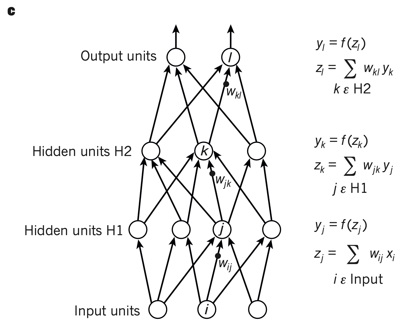
In practice, training samples are supplied as “batches”, however, for illustrative purposes, let us consider the processing of a single training data point, following Figure 1 of LeCun et al., 2015².

• During the forward pass, we compute the activity of each node of each layer as a weighted sum of its inputs, transformed by an activity function.

  For example, to get the ouput of a node $j$ at hidden layer $H1$, we first compute a weighted sum of its three inputs:

  $z_j=\sum_{i \in I} w_{ij}x_i$

  and pass the result in an activation function to get the activity of the node (usually written as $a_j$, here written $y_j$ in Figure c):

  $y_j=f_j(z_j)$

  The activity at all nodes of a layer forms an activity vector which is used as an input layer for nodes of subsequent layers: nodes of layer $H2$ compute weighted sums of the activity vector $y^{H1}$ of layer H1. Nodes of the output layer compute weighted sums of the activity vector $y^{H2}$ to output a bidimensional vector of values (the Output units below):

  

  Our goal when training a neural network is to optimize the weights so that the output of the network corresponds to the target.

• During the backward pass, we adjust the weights of the connections between nodes in the direction that minimizes the prediction error.

  To do this:

  • We evaluate an objective function (also called a cost function or a loss function) which quantifies the error of the actual output of the network relative to the expected output.

    For a regression task (i.e., predicting a continuous value), the square of the residual is used:

    $RS=(y - \hat{y})^2$

    where: $y$ is the target value and $\hat{y}$ is the prediction of the node (sometimes refered to as score of the node)

  • for each node, we compute a formula that gives us the amount of variation in the cost function for a small change in the parameters of the node. That is, we compute the partial derivatives of the cost function relative to each of the parameters of the node.

  

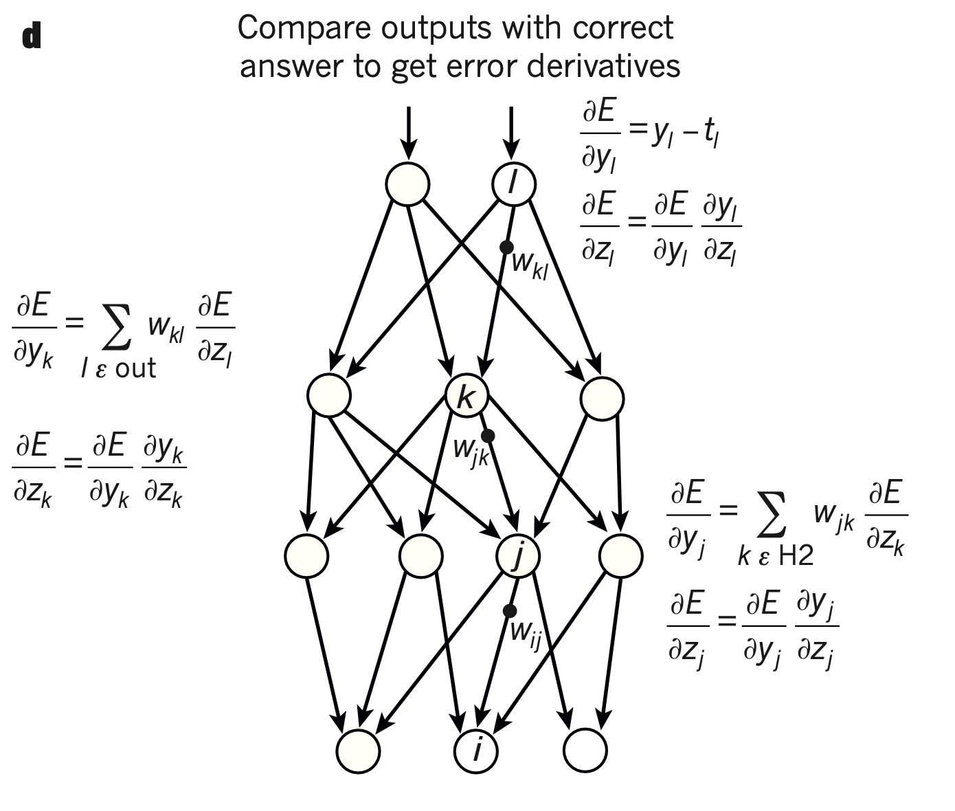
  This procedure is dauntingly termed “backpropagation of the gradient of error” because we start from the most distal node, and use the chain rule of derivatives to compute the partial derivatives of the cost function relative to every parameters further up the network.

  
  
  What is a gradient ?

  
  A gradient is just a vector of partial derivatives of a function with respect to each of its parameters.

  Thus the gradient of the function $z_j$ summing the n=3 inputs $H_1^1$, $H_2^1$ and $H_3^1$ from layer $H1$ at node $j$ can be written:

  $\Delta z_j = \begin{bmatrix}\frac{\partial z_j}{\partial w_{H_1^1j}} \\ \frac{\partial z_j}{\partial w_{H_2^1j}} \\ \frac{\partial z_j}{\partial w_{H_3^1j}}\end{bmatrix}$

  Even though a gradient is technically a vector, the expression “the gradient of x” is used interchangeably with the the technically correct expression “the partial derivative of x with respect to y”, for brevity.

  The following sections are verbose explicitation of Figure 1’s legend of LeCun et al., 2015 Nature review², and worth reading if you are not familiar with neural networks and gradient descent algorithm.

  
  
  Walkthrough on the computation steps required to update weights

  
  

  Our goal is to update the network’s weights by minimizing the error. To achieve this, we aim to compute the partial derivative of the loss function with respect to each weight. We will then use these derivatives to update the weights in a direction that minimizes the error (i.e., in the oppositive direction of the derivatives).

  Here is an example for updating the weight $w_{kl}$ connecting a hidden node $k$ to an output node $l$.

  At each training pass, we update the weight as follows:

  $w_{kl} := w_{kl} - \alpha \frac{\partial E}{\partial w_{kl}}$

  with $\alpha$ the learning rate.

  How do we derive $\frac{\partial E}{\partial w_{kl}}$ ? We will “just” use derivatives rules to compute, step by step, the derivative of the composition of functions that maps $w_{kl}$ to the cost function $E$.

  For a neater derivation expression, we scale the cost function by $\frac{1}{2}$. We also substitute $y$ for $t_l$ (the target value), and $\hat{y}$, the output of our final node, by $y_l$, the notation used in Figure d:

  $RS=\frac{1}{2}(t_l - y_l)^2$

  We express the derivative of the cost function expression with respect to $w_{kl}$:

  $\frac{\partial E}{\partial w_{kl}} = \frac{\partial }{\partial w_{kl}} \frac{1}{2}(t_l - y_l)^2$

  Then, applying the chain rule gives us:

  $\frac{\partial E}{\partial w_{kl}} = \frac{1}{2}*2*(t_l - y_l) \frac{\partial }{\partial w_{kl}}(t_l - y_l)$

  Simplifying and injecting the equation $y_l = f_l(z_l)$ gives us:

  $\frac{\partial E}{\partial w_{kl}} = (t_l - f_l(z_l)) \frac{\partial }{\partial w_{kl}}(t_l - f_l(z_l))$

  Applying the sum rule, we can write:

  $\frac{\partial E}{\partial w_{kl}} = (t_l - f_l(z_l)) (\frac{\partial }{\partial w_{kl}} t_l - \frac{\partial }{\partial w_{kl}} f_l(z_l))$

  The derivative of a constant being 0, this simplifies as:

  $\frac{\partial E}{\partial w_{kl}} = - (t_l - f_l(z_l)) \frac{\partial }{\partial w_{kl}} f_l(z_l)$

  Applying the chain rule again:

  $\frac{\partial E}{\partial w_{kl}} = - (t_l - f_l(z_l)) \frac{\partial f_l(z_l)}{\partial z_l} \frac{\partial z_l}{\partial w_{kl}}$

  If the ouput layer is a multiregression layer, i.e., $f_l$ is the identify function, then $\frac{\partial f_l(z_l)}{\partial z_l} = 1$ and the expression simplifies to:

  $\frac{\partial E}{\partial w_{kl}} = - (t_l - z_l) \frac{\partial z_l}{\partial w_{kl}}$

  Injecting the expression of $z_l$ in the equation:

  $\frac{\partial E}{\partial w_{kl}} = - (t_l - z_l) \frac{\partial }{\partial w_{kl}} \sum_{k \in H2} w_{kl} y_k$

  When deriving the weighted sum with respect to one of the weight, all the other weights are treated as constants and hence the final expression:

  $\frac{\partial E}{\partial w_{kl}} = - (t_l - z_l) \frac{\partial }{\partial w_{kl}} w_{kl} y_k \\ = - (t_l - z_l)y_k$

  The weight will be updated in proportion of the input $y_k$ and the magnitude of deviation from the target $(t_l​ − z_l​)$.

  
  
  The backpropagation algorithm

  
  

  As stated by LeCun et al., “the backpropagation procedure to compute the gradient of an objective function with respect to the weights of a multilayer stack of modules is nothing more than a practical application of the chain rule for derivatives.”.

  During backpropagation, we start by computing the error derivative relative to the end node inputs, and store the intermediate calculations to continue propagating the error derivatives further up the network.

  For an enlightning walkthrough into the matrix implementation of backpropagation, I recommend reading this excellent blog post³ of Brent Scarff. For a visually compelling illustration of backpropagation, follow this video⁴. For a deep dive into the linear algebra intricacies, follow along Chapter 2⁵ of Neural Network and Deep Learning by Michael Nielson. Sebastian Raschka also has a very good didactic post⁶ on backpropagation in artificial neural networks.

  For the purpose of the current article, I will just extend my casual, down to earth example initiated above to illustrate the logic of backpropagation.

  If we now want to update the weights of the last hidden layer, i.e., compute $\frac{\partial E}{\partial w_{jk}}$, we must evaluate the following expression:

  $\frac{\partial E}{\partial w_{jk}} = \frac{\partial E}{\partial y_{k}} \frac{\partial y{k}}{\partial z_{k}} \frac{\partial z{k}}{\partial w_{jk}}$

  The sole additional complication for a connected hidden node (a “deep” node) is that the derivative of the loss function with respect to the ouput of the node depends on the error derivative of all the downstream nodes it connects to.

  For a node $k$, that is: $\frac{\partial E}{\partial y_{k}} = \sum_{l \in out} \frac{\partial E}{\partial y_{l}} \frac{\partial y_{l}}{\partial z_{l}} \frac{\partial z_{l}}{\partial y_{k}}$

  As $\frac{\partial z_{l}}{\partial y_{k}} = \frac{\partial }{\partial y_{k}} \sum_{k \in H2} w_{kl} y_k = w_{kl}$, we obtain:

  $\frac{\partial E}{\partial y_{k}} = \sum_{l \in out} \frac{\partial E}{\partial y_{l}} \frac{\partial y_{l}}{\partial z_{l}} w_{kl}$

  Reinjecting it in the above expression gives us:

  $\frac{\partial E}{\partial w_{jk}} = \sum_{l \in out} \frac{\partial E}{\partial y_{l}} \frac{\partial y_{l}}{\partial z_{l}} w_{kl} \frac{\partial y{k}}{\partial z_{k}} \frac{\partial z{k}}{\partial w_{jk}}$

  As shown in the walkthrough above, $\frac{\partial z{k}}{\partial w_{jk}} = y_j$ and this expression becomes:

  $\frac{\partial E}{\partial w_{jk}} = \sum_{l \in out} \frac{\partial E}{\partial y_{l}} \frac{\partial y_{l}}{\partial z_{l}} w_{kl} \frac{\partial y{k}}{\partial z_{k}} y_j$

  The evaluation of this expression depends on the loss and activation functions used at nodes $l$ and $k$.

  Compared to the single walkthrough outlined above, the backpropagation of gradient of error algorithm consists in computing the gradients of error at each layer (e.g., for hidden layer $H2$, we compute $\delta^z = \begin{bmatrix}\frac{\partial E}{\partial z_{1}} \\ \frac{\partial E}{\partial z_{2}} \\ \frac{\partial E}{\partial z_{3}}\end{bmatrix}$)

  These gradients are computed once during the backward pass, stored, and reused for all upstream calculations.

  As we showed, computing the derivatives with respect to the weights of the final layer is straightforward:

  $\frac{\partial E}{\partial w_{kl}} = \frac{\partial E}{\partial z_{l}} y_{k}$

  For the last hidden layer, it is a bit more involved, and depends on the error derivative at the nodes downstream:

  $\frac{\partial E}{\partial w_{jk}} = \sum_{l \in out} \frac{\partial E}{\partial y_{l}} \frac{\partial y_{l}}{\partial z_{l}} w_{kl} \frac{\partial y{k}}{\partial z_{k}} y_j$

  We can express it as a function of the derivative of the loss function with respect to the weighted sum of inputs of the node:

  $\frac{\partial E}{\partial w_{jk}} = \frac{\partial E}{\partial z_{k}} y_{j}$

  In plain english, as we progress upwards, we multiply the derivative of the loss function with respect to the output of the node, by the derivative of the activation function of the node. This yields the derivative of the loss function with respect to the weighted sum of inputs $\frac{\partial E}{\partial z}$ at the node.

  This term is used:

  • to compute the derivative of the loss function with respect to the weights connecting the node with nodes of the previous layer, e.g., $\frac{\partial E}{\partial w{ij}} = \frac{\partial E}{\partial z_{j}} y{i}$.
  • to continue propagating the error gradient further up the network.

Given a demanding machine learning problem, we devise a deep learning architecture to map an input layer of data features to an output layer comprising one or more output nodes.

The architectural choices of the inner layers is pretty much free ; yet choosing the proper final layer, activation function and loss function depend on the predictive task of the network:

• For a regression task (i.e., predicting one or several continuous values), we use the Mean Absolute Error (MAE) or Mean Squared Error (MSE) loss. Fundamentally, this is “just” optimization by means of gradient descent instead of ordinary least square.
• For a binary classification task (i.e., distinguishing between two classes), we use a single output node with the Sigmoid activation function, and the Binary Cross-Entropy criterion as a loss function.
• for a multi-class classification task (i.e., distinguishing between several classes), we use multiple nodes with the Softmax activation function and the Cross-Entropy criterion as the loss function.

The Pytorch API has dedicated classes which exposes these last two combinations of activation / loss functions as unified logical blocks: nn.BCEWithLogitsLoss and nn.CrossEntropyLoss.

Why do we need to use different activation / loss function combinations in classification tasks?

Well, it turns out we need not to:

• If you train a neural network on a binary classification task using MSE or MAE loss, your network will still manage to learn something, albeit more slowly.
• If you train a neural network on a multi-class classification problem with a sigmoid activation function, your network will learn just fine. But you may ask why use the softmax activation function at all, then ?

We shall see, however, that using the correct combination of activation / loss functions in classification tasks:

1. increases training performance
2. improves interpretability of the network’s output

As it is often the case with statistics or machine learning topics, we can build an intuition of these phenomenons, but fully grasping it will require us to dig into the derivatives to actually verify our gut feelings.

In classification tasks, we seek to assign one (multi-class classification) or several (multi-label classification) labels to a data point given its feature array.

We will first consider the most simple multi-class classification task.

For a binary classification task, our network is tasked to predict a discrete label (yes / no) from a feature vector.

Transforming our two discrete categories into a numerical array that can be used in gradient descent is quite straightforward: we can just assign a positive value (1) to the positive label, and 0 otherwise.

Let us imagine that we train one of the final node $l$ from above to predict 0 or 1. In order to calculate our loss, we need to map the result of the computation accomplished by the node (that is, a weighted sum of its inputs) between 0 or 1.

The most obvious solution is to use a step function, for example cutting the domain in half to output 1 if the weighted sum is positive, and 0 otherwise:

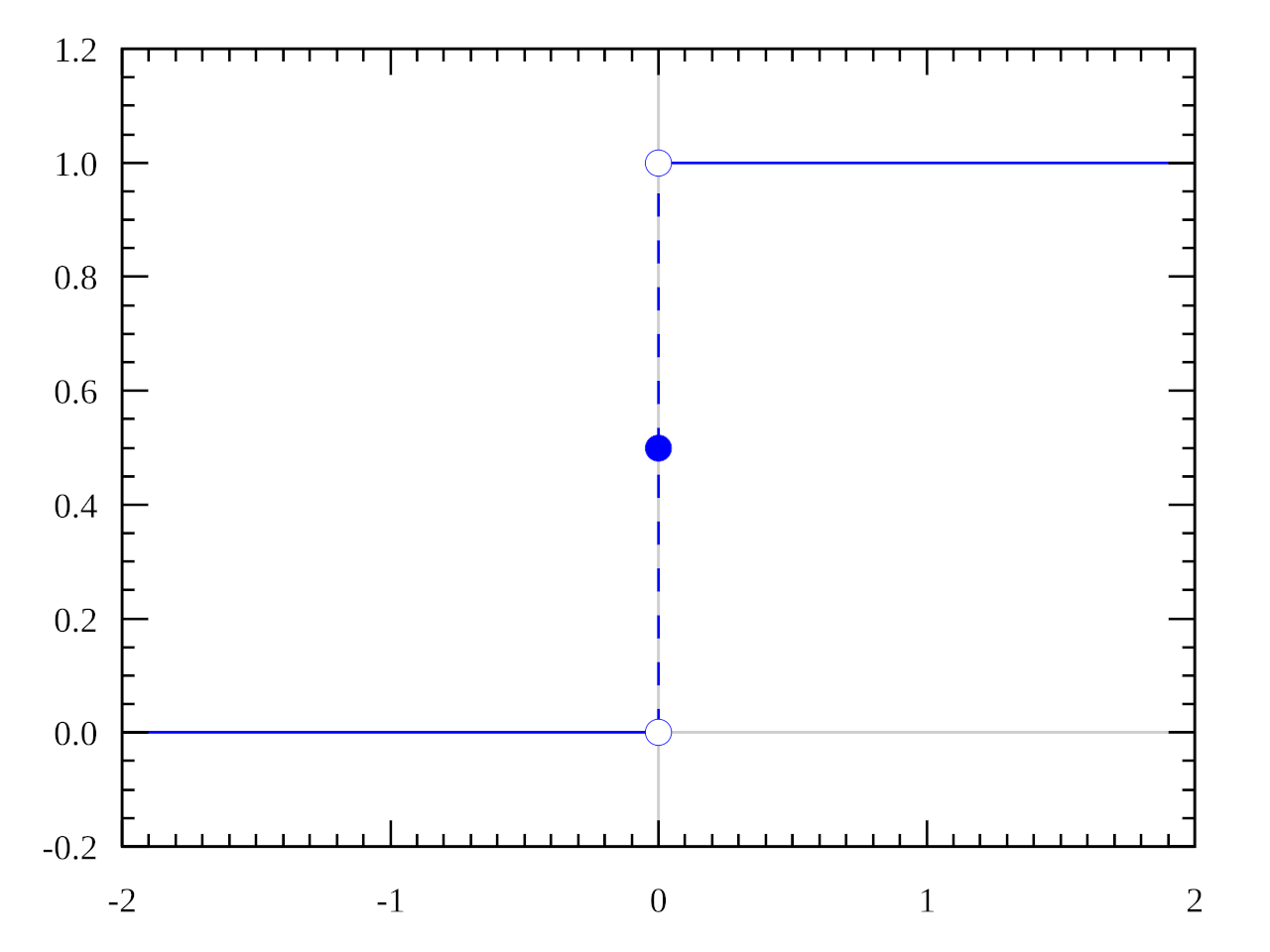
This activation function, called a step function, is used by the perceptron, the most ancient single layer single neuron “network” for supervised learning.

Leveraging the output of this function to measure the performance of our network is straightforward: the loss should be equal to 0 when ground truth and predicted label coincide, and positive otherwise. Thus, the residual square loss, which quantifies the discrepancy between predictions and ground truths in regression tasks can also be used in our classification task:

$RS=(y - \hat{y})^2$

However, there is a big problem with using a step function as an activation function in a neural network: it has a gradient of 0 everywhere (except at x=0, where the function is not defined and its derivative is infinite).

This means that the rate of change in the output of the step function is constant with respect to the changes in the node parameters in the two subdomains where it is defined ($z < 0$ and $z > 0$). Thus, the error derivative of the output node with respect to $z$ (the weighted sum of inputs at the node) will always be 0, and backpropagation will never update any weights in our network !!

The only error signal that can be extracted from a step function is the label discrepancy itself: this is the error measurement used by the perceptron rule⁷.

Instead, we want to use a differentiable activation function, whose variation in output reflects small changes in the weighted sum of inputs.

This is precisely the behaviour of the sigmoid activation function:

$\sigma(z) = \frac{1}{1 + e^{-z}}$

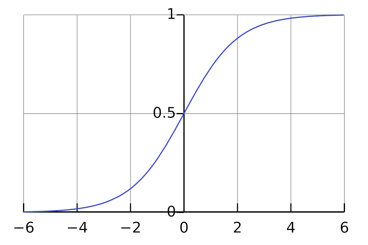
We can see that when $z → -\infty$, $\sigma(z) → 0$ and when $z → +\infty$, $\sigma(z) → 1$

The sigmoid function is differentiable⁸:

$\frac{\partial \sigma (z)}{\partial (z)} = \sigma(z)(1-\sigma(z))$

So we can compute the derivative of the loss function with respect to the network’s weights.

Walkthrough of the derivation of the residual square error function with respect to output node parameters

We start again from this equation:

$\frac{\partial E}{\partial w_{kl}} = - (t_l - f_l(z_l)) \frac{\partial f_l(z_l)}{\partial z_l} \frac{\partial z_l}{\partial w_{kl}}$

If the ouput node $k$ is now a sigmoid-activated node, i.e., $f_l$ is the sigmoid function, we have:

$\frac{\partial E}{\partial w_{kl}} = - (t_l - \sigma(z_l))\sigma(z_l)(1-\sigma(z_l))y_k$

This means the weight will be updated in proportion of the input $y_k$, the magnitude of deviation from the target $(t_l​ − \sigma(z_l)​)$, and the derivative of the sigmoid function with respect to $z_l$, $\sigma(z_l)(1-\sigma(z_l))$.

There is yet a difficulty when using this function with backpropagation: it saturates.

For an output close to 0 or 1, the sigmoid curve flattens, which means mathematically that the gradient (the blue curve on the figure below) gets small:

As the derivative of the loss function with respect to $w_{kl}$ can be expressed as:

$\frac{\partial E}{\partial w_{kl}} = - (t - \sigma(z_l))\frac{\partial \sigma(z_l)}{\partial z_l} y_k$

We can distinguish between two cases during a training pass:

• The discrepancy between predicted label and ground truth is small (i.e., the network predict near 0 for a negative sample and near 1 for a positive sample): $(t - \sigma(z_l)) → 0$, and $\frac{\partial E}{\partial w_{kl}} → 0$. There is little update of the weights, this is the appropriate behaviour.
• The discrepancy between predicted label and ground truth is very big (i.e., the network predict 0 for a positive sample and 1 for a negative sample). Although the absolute value of the first term of the equation tends to 1 ($|(t - \sigma(z_l))| → 1$), $\frac{\partial \sigma(z_l)}{\partial z_l} → 0$, because we are in the “floor” (if $\sigma(z_l)→0$) or “ceiling” (if $\sigma(z_l)→1$) zone of the sigmoid function.

So the further our prediction from the ground truth, the smaller the derivative of the loss function with respect to the weights, and thereby the smaller the weight update by gradient descent !!

This is exactly the opposite of our goal: ideally, we would like a big margin of error to lead to a big correction of the weight.

To remedy this problem of learning saturation, we need a cost function that penalizes the network in proportion of the deviation of the prediction from ground truth.

A way to approach this is to quantify the similarity between the distribution of predicted probabilities of the label by the final node, and the distribution of the “true” probability of the label (that is, 0 or 1).

And there enters the Cross-Entropy (CE) criterion:

$H(p,q) = -\sum_x^n p(x) \cdot \log(q(x))$

This formula calculates the cross-entropy between two probability distributions $p$ and $q$:

• $p(x)$ is the true probability of an event $x$, which we want to predict.
• $\log q(x)$ is the logarithm of the predicted probability of the same event $x$ by our model.
• The sum of this product is taken over all events.

Although this has a profound meaning in information theory⁹, it is rather abstruse as such.

Yet it is surprisingly effective for defining cost functions in classification tasks, as we shall see in the next sections.

The Binary Cross-Entropy (BCE) function is an application of the cross-entropy criterion for the definition of the loss of a binary classifier:

$\mathcal{L}_{BCE} = -\frac{1}{n} \sum_x^n(y \cdot \log(\hat{y}) + (1 - y) \cdot \log(1 - \hat{y}))$

This loss computes the sum of the cross-entropy criterion between the distribution of true and predicted probabilities of a positive ($y$) and negative ($1-y$) label, averaged across $n$ training samples.

Although this expression may be difficult to grasp at first sight, plugging in some toy examples of maximal label and ground truth discrepancies is easy:

• when $y = 1$ and $\hat{y} = 0$, then $\mathcal{L}_{BCE} = - (y \cdot \log(\hat{y})) → +\infty$
• when $y = 0$ and $\hat{y} = 1$, then $\mathcal{L}_{BCE} = (1-\hat{y}) \cdot \log(1 - y) → +\infty$

Conversely, when $\hat{y}$ and $y$ agree, $\mathcal{L}_{BCE} → 0$

Intuitively, this cost function solves the problem poised by the saturation of the sigmoid function. We can verify this by working out the derivatives of the binary cross-entropy with respect to the weights of the network:

Walkthrough of the derivation of the cross-entropy loss function with respect to output node parameters

By substituting the residual square loss function with the cross-entropy loss in the expression of the error derivative with respect to the weight $w_{kl}$, plugging in $\hat{y} = \sigma(z_l)$ and $y = t$ we obtain:

$\frac{\partial E}{\partial w_{kl}} = \frac{\partial }{\partial y_l} - (t \cdot \log(\sigma(z_l)) + (1 - t) \cdot \log(1 - \sigma(z_l))) \frac{\partial \sigma(z_l)}{\partial z_l} y_k$

Taking the derivative of the logarithm and applying the difference rule of derivative bring us to:

$\frac{\partial E}{\partial w_{kl}} = (- \frac{t}{\sigma(z_l)} + \frac{1 - t}{1 - \sigma(z_l)})\frac{\partial \sigma(z_l)}{\partial z_l} y_k$

Working a common denominator and simplifying:

$\frac{\partial E}{\partial w_{kl}} = \frac{- t(1 - \sigma(z_l)) + (1-t)\sigma(z_l)}{\sigma(z_l)(1 - \sigma(z_l))}\frac{\partial \sigma(z_l)}{\partial z_l } y_k \\ = \frac{\sigma(z_l) - t}{\sigma(z_l)(1 - \sigma(z_l))}\frac{\partial \sigma(z_l)}{\partial z_l} y_k$

Injecting the derivative of the sigmoid function with respect to the sum of inputs gives us:

$\frac{\partial E}{\partial w_{kl}} = \frac{\sigma(z_l) - t}{\sigma(z_l)(1 - \sigma(z_l))} \sigma(z_l)(1-\sigma(z_l)) y_k$

Which simplifies to:

$\frac{\partial E}{\partial w_{kl}} = (\sigma(z_l) - t) y_k$

In plain english, this means that the derivative is proportional to $(\sigma(z_l) - t)$: the greater the discrepancy between prediction and ground truth, the stronger we update the weight. This makes perfect sense.

Moreover, the cross-entropy loss function eliminates the dependency of the gradient of error on the sigmoid derivative, thus avoiding learning saturation.

The binary cross-entropy cost function can easily be generalized to a multi-class or multi-label paradigm using an output layer with more than one node.

• In multi-class classification, we seek to predict one exclusive label out of $C$ classes. The target vector $t$ is a one-hot vector of size $C$ with a 1 (encoding the positive class) and $C−1$ 0s (encoding the negative classes).

• In multi-label classification, we seek to predict -possibly- more than one labels from a set of non-exclusive $C$ classes. The target vector $t$ is a vector of size $C$ of 0s and 1s.

For such tasks, we design the final output layer with as many nodes as they are classes: each node encodes the probability of the data point belonging to the corresponding class $t_l$.

The proper cost function will differ however, given the task.

In multi-label classification, predictions are independent, so we just have to sum the binary cross-entropy costs across all nodes to calculate our total error:

$\mathcal{L}_{CE} = -\frac{1}{n} \sum_x^n \sum_{l \in out} [t_l \log \hat{y_l} + (1-t_l) \log (1-\hat{y_l}) ]$

And use this error to optimize the weights.

Derivation of the multi-label cross-entropy loss function with respect to output node parameters

$\frac{\partial E}{\partial w_{kl}} = \frac{\partial }{\partial y_l} -\sum_{l \in out} [(t \cdot \log(\sigma(z_l)) + (1 - t) \cdot \log(1 - \sigma(z_l)))] \frac{\partial \sigma(z_l)}{\partial z_l} y_k$

When deriving with respect to a node output $y_l$, all the other outputs are treated as constants and we fall back on the expression of the error derivative for a single output node network:

$\frac{\partial E}{\partial w_{kl}} = (\sigma(z_l) - t) y_k$

Given a data point, the score of each node of the output layer will encode the probability estimate of the corresponding label.

In multi-class classification, we train the network to assign each data point to the unique class it belongs to.

Optimizing the binary cross-entropy cost function across several nodes as in the multi-label paradigm will work just fine, but is suboptimal when it comes to interpreting our network’s output.

Indeed, the vector of probabilities concatenated from the output nodes can not be interpreted as the network’s estimate of correct class probability:

• The predictions do not sum to 1.
• The relative score of the output nodes can not be jointly interpreted: the output of each nodes are independently trained in as many binary classification tasks as they are of possible target classes.

So we need to:

1. Extend the cross-entropy cost function to handle multiple (C > 2) classes.
2. Constrain the prediction layer into representing a vector of probabilities over mutually exclusive targets.

Extending cross-entropy to handle $C > 2$ classes is straightforward:

$\mathcal{L}_{CE} = -\frac{1}{n} \sum_x^n \sum_i^C y_i \log(\hat{y_i})$

Where $y_i$ and $\hat{y_i}$ are the ground truths and the predictions of the output node for each class $i$ in $C$.

As only one class is possible for each sample, the formula simplifies to $\mathcal{L}_{CE} = -\frac{1}{n} \sum_x^n \log(\hat{y})$, where $\log(\hat{y})$ is the log of the probability of the correct class.

However, we can not directly apply this formula to the output layer of sigmoid-activated nodes:

Derivation of the multi-class cross-entropy loss function with respect to output node parameters

We note $t_l$ the target’s label of node $l$:

• if $t_l = 1$:

  $\frac{\partial E}{\partial w_{kl}} = - \frac{\partial }{\partial y_l} \log(y_l) \frac{\partial y_l}{\partial w_{kl}}$

  $\frac{\partial E}{\partial w_{kl}} = \frac{1}{\sigma(z_l)} \sigma(z_l)(1-\sigma(z_l))y_k \\ = (1-\sigma(z_l))y_k$

• if $t_l = 0$, $\mathcal{L}_{CE} = 0$ and $\frac{\partial E}{\partial y_l} = 0$, nothing happens at the node.

Thus, using this cross-entropy formulation with one-hot vector targets will only update the weights of the node predicting the probability of the target class. This means that:

• There is no warranty for the target’s output node to have the higher score, i.e., the network does not control for false positive predictions by off-target nodes, making the system unreliable.
• The vector of scores given a feature array is even more problematic to interpret.

To constrain the prediction layer into representing a vector of probability across mutually exclusive targets, a final piece of computational refinement is used, the softmax activation function:

$y_l = \frac{e^{z_l}}{\sum_{l \in out} e^{z_l}}$

In plain english, this boils down to normalizing the activity of each output node by the sum of the activity over the entire output layer.

The most appealing property of this transformation is that it converts the raw scores (or “logits”) at the output of the final nodes into a probability distribution (i.e., a vector that sums to 1). This is handy because it allows us to interpret predictions of the final nodes as the network’s estimate of the probability that the correct output is $C$.

💡 You will often read the term “logits” for the outputs of a classification model. It refers to the vector of raw, untransformed outputs of the final layer ($z_l$) before they are passed into a normalization function (sigmoid or softmax).

• In a binary classification problem, the logit is the $z_l$ ($l = 1$) input of the single final node which is passed to the sigmoid activation function.
• In a multi-class classification problem, logits are the $z_l$ ($l = n_{classes}$) inputs to the softmax function.

The softmax activation function should actually be called softargmax. Softmax can indeed be considered a “soft” version of the argmax function: Instead of returning a 1 at the position of the maximum element in the $z$ vector, and 0 for the rest, it returns the highest value at the position of the maximum element, and small values for the rest of the vector.

The use of the exponential function ensures that:

• Every output value is positive.
• The largest components in the input vector remains the largest in the output vector.
• The normalization function is differentiable, enabling the seamless application of the chain rule for the computation of the error derivative during backpropagation.

Injecting the formula for softmax normalization in the cross-entropy loss function, we can write:

$\mathcal{L}_{CE} = -\frac{1}{n} \sum_x^n \sum_i^C y_i \log(\frac{e^{z_l}}{\sum_{l \in out} e^{z_l}})$

The combination of the softmax activation function with the cross-entropy loss is refered to as the Categorical Cross-entropy loss. Computing its derivative is a bit more involved than what we did up to now, because it depends:

• On the output node we want to find the derivative for (in an analogous way to the walkthrough above, where we considered the derivative of the loss function at the node predicting the probability of the positive class, versus all the other nodes where it equals 0).
• With respect to which input of the softmax function we want to compute the derivative of the loss function of the node.

There are lots of bits and pieces over the internet exposing the derivation of the softmax and cross-entropy loss functions ; but they are often hard to follow because they all use different notation conventions, derivation steps, and math junkies tricks. The most rigorous and comprehensive exploration of the matter I could find is on Eli Bendersky’s site¹⁰

In the section below, I walk through a down to earth derivation of the categorical cross-entropy loss function applied to our dual output node network.

In the end, we show that the derivative of the loss function with respect to the weights of the network is identical to applying the binary cross entropy across sigmoid-activated nodes.

Walkthrough of the derivation of the categorical cross-entropy loss function with respect to output node parameters

As previously, we are interested in computing the derivative of the loss function with respect to the weight $w_{kl}$.

Using the chain rule to express the derivative of the cost function with respect to the weight $w_{kl}$, we can write:

$\frac{\partial E}{\partial w_{kl}} = \frac{\partial E}{\partial z_{l}}\frac{\partial z_{l}}{\partial w_{kl}}$

The important point to note when using the softmax activation function is that the gradient of the output of any node $y$, depends on the weighted sum of inputs $z$ of all other output nodes. So we need to use different node subscripts to distinguish between before and after softmax activation nodes. We introduce $c$, which identify the index of the class.

The derivative of the cross-entropy loss with respect to the sum of inputs of the node $l$ is:

$\frac{\partial E}{\partial z_l} = \frac{\partial }{\partial y_c} - \sum_c^C t_i\log y_c$

Applying the chain rule, we obtain:

$\frac{\partial E}{\partial z_l} = - \sum_c^C t_c \frac{1}{y_c} \frac{\partial y_c}{\partial z_l}$

We want to compute the derivative of the softmax output at node $c$ with respect to the sum of inputs at node $l$. For clarity, I will condense the denominator of the softmax $\sum_{l \in out} e^{z_l}$ into $\sum$.

$\frac{\partial y_c}{\partial z_{l}} = \frac{\partial }{\partial z_{l}} \frac{e^{z_l}}{\sum}$

We need to distinguish between two cases:

• if $c = l$:

  Using the quotient rule, we get:

  $\frac{\partial y_c}{\partial z_{l}} = \frac{e^{z_c} \sum - e^{2z_c}}{\sum ^2}$

  [Hints: $(e^{x})' = e^x$ and $e^{x}.e^{x} = e^2x$]

• if $c ≠ l$:

  During derivation, $e^{z_l}$ is treated as a constant and applying the quotient rule gets us to:

  $\frac{\partial y_c}{\partial z_l} = \frac{- (e^{z_c}e^{z_l})}{\sum ^2}$

We can now compute the derivative of the cross-entropy loss with respect to $z_l$. First we take the derivative of the log:

$\frac{\partial E}{\partial z_l} = - \sum_c^C t_c \frac{1}{\frac{e^{z_c}}{\sum}} \frac{\partial y_c}{\partial z_l} \\ = - \sum_c^C t_c \frac{\sum}{e^{z_c}} \frac{\partial y_c}{\partial z_l}$

We can now inject our two equations of the derivative of the softmax output with respect to inputs into the expression.

Note that for the $c = l$ condition, we use the $l$ subscript:

$\frac{\partial E}{\partial z_l} = - (t_l \frac{\sum}{e^{z_l}} \frac{e^{z_l} \sum - e^{2z_l}}{\sum ^2} + \sum_{c≠l} t_c \frac{\sum}{e^{z_c}} \frac{- (e^{z_c}e^{z_l})}{\sum ^2})$

This expression simplifies to:

$\frac{\partial E}{\partial z_l} = - (t_l \frac{\sum - e^{z_l}}{\sum } - \sum_{c≠l} t_c \frac{e^{z_l}}{\sum }) \\ = - (t_l (1 - \frac{e^{z_l}}{\sum }) - \sum_{c≠l} t_c y_l) \\ = -(t_l(1 - y_l) - \sum_{c≠l} t_c y_l) \\ = - t_l(1 - y_l) + \sum_{c≠l} t_c y_l \\ = - t_l + t_ly_l + \sum_{c≠l} t_c y_l$

If we reintegrate $t_ly_l$ in the sum over all nodes $c$, we get:

$\frac{\partial E}{\partial z_l} = - t_l + \sum_{c}^C t_c y_l$

Given that the one-hot vector sums to one, $\sum_{c}^C t_c = 1$ and we arrive to the final expression:

$\frac{\partial E}{\partial z_l} = y_l - t_l$

Closing the loop, if we express $y_l$ as $\sigma(z_l)$:

$\frac{\partial E}{\partial w_{jk}} = \frac{\partial E}{\partial z_l} \frac{\partial z_l}{\partial w_{jk}} \\ = (\sigma(z_l) - t_l)y_k$

Which is equivalent to the expression we derived from multi-node binary cross-entropy loss.

Thus, using the categorical cross-entropy loss:

• transforms the network’s output into an estimate of the correct class probability among multiple mutually exclusive classes.
• avoids learning saturation.

And there ends our journey through the activation and loss functions used in neural network classifiers.

We covered:

1. The principles of feed-forward and backward passes in neural networks.
2. How the backpropagation algorithm is used to optimize the weights of a neural network.
3. The rational behind the sigmoid activation function used in classification tasks.
4. Why the cross-entropy loss function avoids learning saturation caused by the sigmoid function.
5. How the combination of softmax activation and cross-entropy loss functions allow for optimal learning and interpretability of the predictions of neural network classifiers.

---

Footnotes

Section titled [object Undefined]

1. The curse of dimensionality, Wikipedia ↩

2. Deep Learning, Nature review ↩ ↩² ↩³

3. Understanding Backpropagation, by Brent Scarff on Medium ↩

4. Backpropagation calculus, 3Blue1Brown on Youtube ↩

5. How the backpropagation algorithm works, in Neural Networks and Deep Learning by Michael Neuser ↩

6. How to compute gradients with backpropagation for arbitrary loss and activation functions?, by Sebastian Raschka ↩

7. What is the difference between a Perceptron, Adaline, and neural network model?, by Sebastian Raschka ↩

8. Derivative of the sigmoid function, on StackOverflow ↩

9. Qualitively what is Cross Entropy ?, on StackOverflow ↩

10. The Softmax function and its derivative, by Eli Bendersky ↩